Start of topic | Skip to actions
3D Euler equations - Explosion in a Box
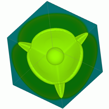
3 Grid Levels (density, isosurface at 1.8)
Results:
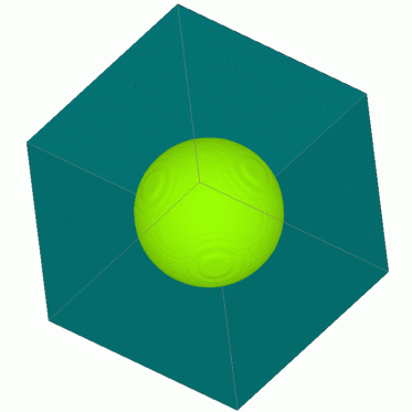 | 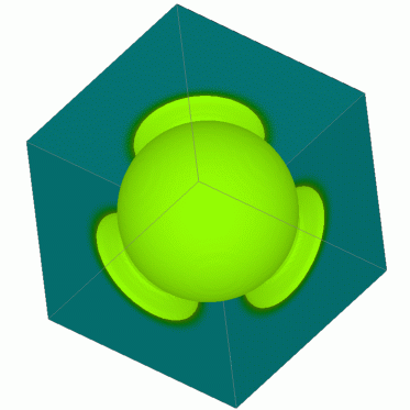 |  | ||
| t=0 | t=0.125 | t=0.25 |
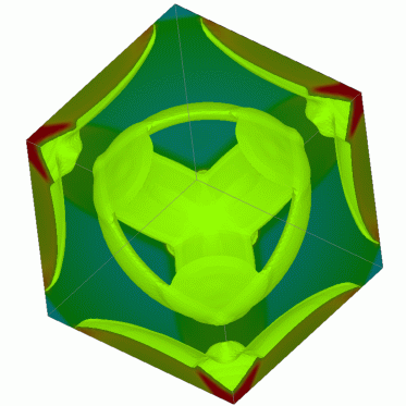 | 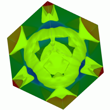 | |
| t=0.375 | t=0.5 |
Benchmark
Adaptive computation with 3 grid levels
| Task | P=1 | P=2 | P=4 | |||
| s | % | s | % | s | % | |
| Integration | 26392 | 94.7 | 12486 | 84.3 | 6166 | 79.3 |
| Flux correction | 428 | 1.5 | 670 | 4.5 | 423 | 5.4 |
| Boundary setting | 233 | 0.8 | 1066 | 7.2 | 809 | 10.4 |
| Recomposition | 402 | 1.4 | 323 | 2.2 | 207 | 2.7 |
| Clustering | 165 | 0.6 | 93 | 0.6 | 52 | 0.7 |
| Misc. | 250 | 0.9 | 171 | 1.2 | 109 | 1.5 |
| Total / Parallel Efficiency | 27870 | 100.0 | 14810 | 94.1 | 7766 | 89.7 |
|---|---|---|---|---|---|---|
Uniform refinement
| Task | P=1 | P=2 | P=4 | |||
| s | % | s | % | s | % | |
| Integration | 74957 | 99.1 | 16884 | 80.8 | 8418 | 97.7 |
| Flux correction | 0 | 0.0 | 0 | 0.0 | 0 | 0.0 |
| Boundary setting | 15 | 0.0 | 105 | 0.5 | 41 | 0.5 |
| Recomposition | 0 | 0.0 | 0 | 0.0 | 0 | 0.0 |
| Clustering | 0 | 0.0 | 0 | 0.0 | 0 | 0.0 |
| Misc. | 634 | 0.9 | 3904 | 18.7 | 145 | 1.8 |
| Total / Parallel Efficiency | 75606 | 100.0 | 20894 | 180.9 | 8604 | 219.7 |
|---|---|---|---|---|---|---|
<--- Problem description
-- RalfDeiterding - 06 Dec 2004